Variability, sampling and data quality

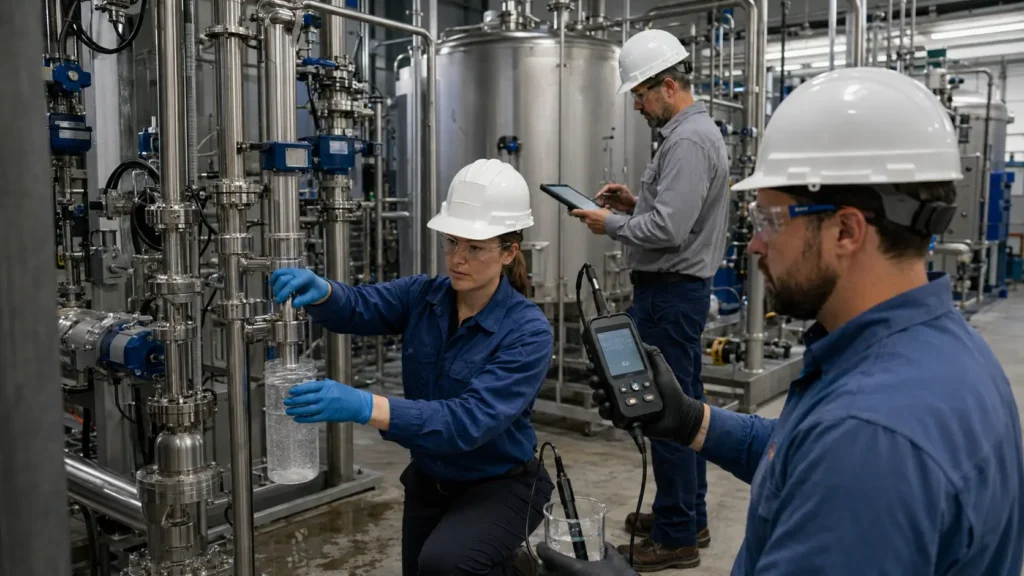
A single analysis is an observation. Design requires a defensible distribution linked to operating states.

Controlled principle Representativeness is not a property of a bottle. It is the relationship between the project decision, the operating states to be represented, the sampling location and duration, the sample type, preservation, method performance and the uncertainty that remains.

7.1 Variability is part of the wastewater definition

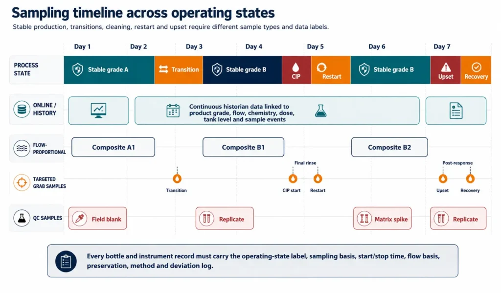
Industrial wastewater varies because the plant varies. Production grade, throughput, feedstock, ore blend, cooling load, evaporation, reagent dose, recycle inventory, tank residence time, membrane recovery, cleaning and operator response can all change flow and composition. Some changes are gradual; others occur as short events that control equalization, peak chemical demand, scaling risk or residual classification.

The sampling objective is therefore not to collect a chemically attractive average. It is to characterize the operating states that the treatment and residual-management system must survive. EPA’s current Quality Assurance Project Plan guidance requires project objectives, sampling design, methods, quality control and data management to be planned together. EPA’s sampling-design guidance similarly begins with the population, spatial or temporal scale and decision that the data must represent. 

For this guide, the population is the wastewater generated within the stated project boundary over the operating modes relevant to design. A normal production composite may be representative of routine annual loading but completely unrepresentative of a two-hour cleaning discharge, a restart flush or a tank-bottom purge. Those events require their own samples and labels.

7.2 Define the inference space before collecting samples

The inference space is the set of conditions to which the project intends to apply the results: particular stream, unit, production grades, campaigns, seasons, flow range, chemical-dose range and event types. USGS quality-control guidance uses the same concept to determine where and when QC samples apply and which environmental samples they can support. 

A sampling plan should be written from an operating-state matrix. Each state needs an occurrence frequency, duration, expected hydraulic range, expected chemistry change, design consequence and sample strategy. States that never co-occur should remain separate; combining independent maxima into one “worst-case” composition can create a feed that the plant never produces.

Operating state	Occurrence and duration	What may change	Sampling basis	Design use
Stable production by grade / campaign	Defined run length and repeat frequency.	Flow, major ions, organics, temperature, additives and product losses.	Flow-proportional composite plus field trends and targeted grabs if needed.	Normal loads, campaign-specific chemistry and routine treatment duty.
Transition between products or feeds	Short, scheduled transition.	Mixed composition, pH/redox shift, solvent or product carryover.	Targeted sequential grabs; do not blend with stable composites.	Equalization, compatibility and transient residual route.
CIP, regeneration or rinse	Batch volume, sequence and frequency.	pH, conductivity, COD/TOC, chelants, oxidants, displaced ions and surfactants.	Separate grabs or event composite by step; preserve unstable analytes separately.	Peak dose, storage, neutralization and batch treatment.
Start-up / shutdown	Defined sequence and drain-down.	Flush water, corrosion products, stagnant inventory and off-spec material.	Timed grabs tied to historian and tank levels.	Contingency routing and short-duration peak load.
Seasonal / utility condition	Warm/cold or dry/wet operating period.	Evaporation, cooling cycles, source-water chemistry and biological activity.	Repeat stable-state programme in each relevant season.	Seasonal operating envelope and materials risk.
Credible upset	Event-specific cause, duration and response.	Spill, dose failure, overflow, pH extreme, solids or oil.	Safe targeted sampling and documented reconstruction from records.	Worst credible contingency, storage and bypass prevention.

Table 7.1. Operating-state matrix: define the inference space before specifying sample count or frequency.

7.3 Grab, time-composite and flow-proportional samples answer different questions

A grab sample is a discrete observation at a defined time and location. It is appropriate for short batch discharges, rapidly changing conditions and analytes that cannot be composited without loss, transformation or cross-contamination. It can identify a peak or process step, but it cannot describe a longer operating period unless the state is demonstrably stable.

A time-proportional composite combines equal aliquots collected at equal time intervals. It estimates the time-average concentration during the compositing period. A flow-proportional composite weights aliquots by flow or collects them after defined discharged volumes; it is normally the more direct basis for average mass loading when flow changes. EPA’s industrial sampling guidance describes these distinctions and notes that the permit, variability, analytical method and sampler compatibility govern the selection. 

Compliance requirements are jurisdiction- and parameter-specific. In the U.S. pretreatment framework, 40 CFR 403.12(g)(3) requires grab sampling for specified unstable or non-compositable parameters and composite sampling for others unless the control authority authorizes an alternative. That rule is a bounded regulatory example, not a universal design recipe. 

Sample type	What it represents	Use when	Do not use when	Minimum metadata
Grab	Conditions at a specific point in time and place.	Short batch, transition, peak, field parameter, volatile/unstable or non-compositable analyte.	The decision requires an average load or a variable operating period.	Exact time, process state, sampler/location, flow and event step.
Time composite	Time-average concentration over the stated period.	Flow and discharge pattern are sufficiently stable for the objective.	Flow varies materially and the decision is mass load; incompatible states or analytes are mixed.	Aliquot volume, interval, start/stop, missed aliquots, refrigeration/preservation and flow record.
Flow-proportional composite	Flow-weighted average concentration and average mass-loading basis.	Flow varies and load or whole-period average is required.	No reliable flow signal exists; the analyte changes in sampler tubing or during storage.	Flow meter ID/quality, triggering rule, aliquot volumes, total represented flow and sampler audit.
Event composite	Defined batch or event, sometimes step-weighted.	CIP, regeneration, tank drain, rainfall or discharge event has a clear beginning and end.	Chemically incompatible steps should remain separate or the event has no reproducible boundary.	Event definition, step sequence, volume per step, mixing basis and unrepresented losses.

Table 7.2. Sample type must match the temporal and hydraulic question.

7.4 Averages depend on how the sample is constructed

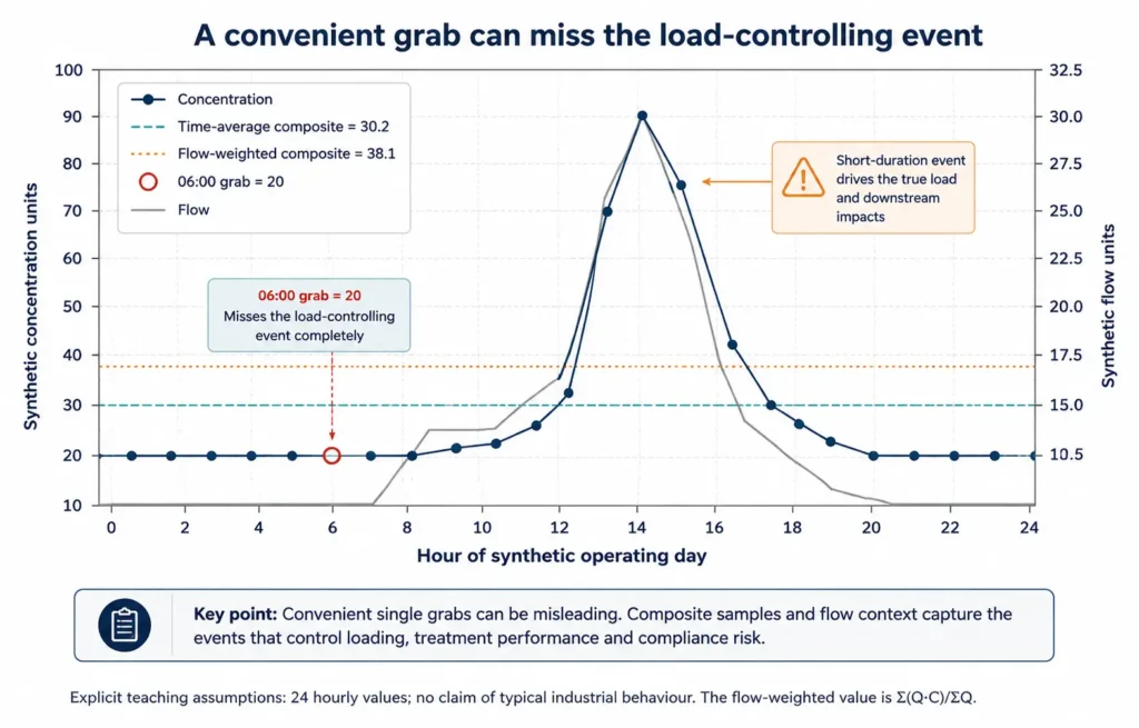
When concentration and flow rise together, a convenient grab and a time-average composite can understate the load-weighted condition. Figure 7.2 uses explicit synthetic hourly values. The 06:00 grab is 20 concentration units, the time-average is 30.3, and the flow-weighted composite is 38.1 because the high-concentration event coincides with high flow. These numbers are a teaching calculation only; they are not industrial benchmarks.

7.5 Preservation and method limits are part of representativeness

The chemistry can change between the process and the instrument. Cooling, aeration, gas loss, oxidation, reduction, precipitation, adsorption, biological activity, volatilization and contact with sampler tubing or bottles can alter the result. Sample handling must therefore be specified before collection, not after the laboratory receives the bottles.

USGS National Field Manual chapters cover preparation, collection, filtration, bottling, preservation, handling and shipping as a connected procedure. For U.S. Clean Water Act compliance data, 40 CFR 136.3 Table II specifies required containers, preservation and maximum holding times by parameter; the applicable method and permit must be checked for the current requirement. The table should not be copied into a general booklet as if one preservation scheme applies to every industrial matrix. 

Parameter behaviour	Sampling / preservation implication	Failure mode	Design response
Rapid field change: pH, temperature, gases, redox	Measure at source or immediately under a documented stabilized condition.	Cooling, aeration or degassing changes speciation and saturation.	Retain field and laboratory values separately; model the treatment temperature and pressure.
Volatile or headspace-sensitive organics	Use method-compatible containers, minimal headspace where required and rapid preservation/transport.	Loss to atmosphere or sampler tubing; cross-contamination.	Use targeted grabs and dedicated equipment; do not rely on a general composite.
Precipitating or adsorbing species	Define filtered/unfiltered fraction, filtration timing, acidification and solids handling.	Precipitation in bottle or dissolution of solids creates a different fraction.	Preserve both dissolved and total/recoverable fractions where the decision needs both.
Biological / reactive demand parameters	Control temperature, holding time and matrix-specific inhibition; use required method.	Biological change or chemical reaction continues after collection.	Plan laboratory receipt around the event; flag any exceedance before interpretation.
Oil, solids and heterogeneous slurries	Mixing, sampler intake and bottle filling must represent the physical phase.	Settling, flotation, wall loss or a blocked intake biases the sample.	Document agitation and collect phase-specific or total-stream samples as required.

Table 7.3. Preservation and method constraints can determine the sample type and collection sequence.

7.6 Quality-control samples quantify contamination, matrix effects and variability

A sampling programme cannot assess its own reliability using environmental samples alone. USGS guidance separates bias and variability and uses blanks, spikes and replicates to estimate them. Blanks evaluate contamination; spikes evaluate method performance and matrix effects; replicates evaluate variability in collection, processing and analysis. The mix and frequency are project-specific and should cover the inference space. 

The QA plan should also define equipment cleaning, calibration, sample custody, laboratory receipt, data validation, corrective action and how failed QC affects the associated environmental results. EPA’s 2025 QAPP guidance treats these as planned elements of the data-generation process, not administrative attachments. 

QC type	Primary question	Where to place it	Interpretive consequence
Equipment blank	Did cleaned equipment, tubing or containers contribute contamination?	Before first use, after difficult matrices or after cleaning changes.	Contamination may qualify or invalidate related low-level results.
Field blank	Did field handling, environment, transport or processing introduce contamination?	Within the same equipment and field sequence as environmental samples.	Defines bias affecting the associated sampling conditions.
Trip blank	Was contamination introduced during transport, especially for volatile targets?	Travels unopened with the sample set.	Qualifies volatile results when transport contamination is detected.
Replicate / split	How variable are collection, mixing, processing and laboratory analysis?	Across different states, concentrations and matrices—not only the easiest sample.	Supports precision estimates and identifies heterogeneous streams.
Matrix spike / spike duplicate	Does the matrix suppress, enhance or degrade target recovery?	Representative high-salinity and high-organic matrices.	Low or erratic recovery limits quantitative use and may require another method/dilution.
Reference / check standard	Is the measurement system calibrated and controlled?	Laboratory and field instrument programme.	Drift or control failure triggers rerun, recalibration or qualification.

Table 7.4. QC samples estimate different error mechanisms; none substitutes for another.

7.7 Cross-check the chemistry before building a design case

A data set should pass independent physical and chemical checks before it enters modelling. The charge-balance error is commonly written as 100 × (Σ cation equivalents − Σ anion equivalents) / (Σ cation equivalents + Σ anion equivalents). PHREEQC can report charge balance and percent error, but the result only tests the ions entered. A poor balance is a diagnostic for omitted species, basis errors, analytical bias or sample change; a good balance does not prove that organics, neutrals, oil or all trace species were measured. 

No universal acceptance percentage is adopted in this guide. The acceptable imbalance depends on salinity, method uncertainty, dilution, analyte list and the decision. Concentrated brines may show small percentage errors that still represent large absolute missing loads, while a low-ionic-strength sample can show a larger percentage from small analytical differences.

Conductivity, density, gravimetric TDS, speciated-ion sums and process chemical additions provide additional checks. They need not match numerically because they measure different properties, but they should tell a coherent story. Disagreement should trigger unit and basis review, dilution verification, method/QC review and targeted reanalysis—not automatic smoothing.

Cross-check	What it can reveal	What it cannot prove	Corrective action
Cation–anion charge balance	Missing major ions, basis conversion errors, dilution or transcription mistakes.	Completeness of neutral organics, gases, oil or uncharged species.	Recalculate on equivalent basis; review alkalinity/carbon, N/S basis and unmeasured ions; resample if needed.
Conductivity versus ion pattern	Inconsistent dilution, temperature correction, gross ion omissions or changed water type.	A universal TDS conversion or product purity.	Check reference temperature, instrument range and major-ion model.
Density versus TDS / ion sum	Impossible mass-volume conversion, unit error or wrong sample identity.	Detailed composition or activity coefficients.	Measure density at stated temperature; convert all loads on one mass/volume basis.
Gravimetric TDS versus speciated ions	Unmeasured dissolved residue, volatile loss, hygroscopic residue or analytical closure issue.	Which missing species explains the difference.	Review methods and matrix effects; retain difference as uncertainty until identified.
Process chemical mass ledger	Unreported acid, base, regenerant, antiscalant, cleaning or neutralization load.	Actual residual speciation or reaction yield.	Reconcile dose records with sample timing and add targeted analyses.
Replicates / time series	Heterogeneity, process variability, sampler or laboratory precision.	Cause of variability without operating-state data.	Link to historian; separate analytical from process variance.

Table 7.5. Cross-checks are diagnostics; they do not authorize invention of missing chemistry.

7.8 Reconstructing a missing ion is a hypothesis, not a measurement

Incomplete historical data are common. Reconstruction can support a screening case when its purpose and uncertainty are explicit, but it must not be presented as laboratory composition. The first task is to correct known reporting-basis errors and identify the process source that could plausibly supply the missing charge or mass.

PHREEQC permits an entered component or pH to be adjusted to achieve charge balance. That is a modelling function, not evidence that the adjusted component was present at the calculated concentration. The selected ion must be chemically and operationally plausible, and the adjusted case should be labelled as an assumption requiring verification. 

Reconstruction level	Permitted use	Required label / evidence	Escalation trigger
1. Basis correction	Correct as N versus NO₃, S versus SO₄, alkalinity basis, density or unit conversion.	Documented source report and visible conversion.	Conflicting certificates or unknown reporting basis.
2. Process-informed inventory	Estimate a known regenerant, neutralization salt or chemical dose for a preliminary balance.	Dose record, stoichiometry, purity, timing and bounded reaction/yield assumption.	Observed conductivity/TDS or ion data do not reconcile.
3. Model charge adjustment	Test sensitivity to one plausible omitted ion or carbon-system variable.	“Assumed for screening—unmeasured”; show original imbalance and adjusted amount.	The assumption changes technology, recovery, product or residual decision.
4. Bounded unknown-ion term	Carry unresolved charge or mass as an explicit unknown range.	Uncertainty register and downside case.	Unknown term is material to dose, scaling, corrosion or product purity.
5. Verification sampling	Replace reconstruction with targeted measurement.	Updated sampling plan, method and operating-state coverage.	Always required before FEED, guarantee or product qualification when material.

Table 7.6. Hierarchy for handling missing ions without converting assumptions into facts.

7.9 Build normal, design and worst-credible compositions from distributions

The project should preserve the observations by operating state and then construct explicit cases. “Normal” describes the representative routine condition for the stated campaign or period. “Design” describes the condition used to size or guarantee a unit, often a selected percentile, upper envelope or co-occurring combination justified by the process. “Worst credible” describes an event that can physically occur within the stated boundary and response time.

These cases are not formed by taking the maximum of every analyte from different dates and combining them. That can violate electroneutrality, mass balance and process reality. The case-building method should identify which variables co-vary, which are independent, and which state controls each equipment or residual decision. USGS QC guidance supports reporting percentiles and confidence intervals where the data support them, while EPA QAPP guidance requires the decision rules and data-quality criteria to be declared in advance. 

Case	Purpose	Construction basis	Do not do	Required output
Normal	Annual mass balance, routine OPEX and stable operation.	State-specific central distribution and flow-weighted load; include availability and frequency.	Average incompatible campaigns or remove genuine routine variability.	Central value plus range/percentiles, frequency and covariance notes.
Design	Hydraulic, chemical, membrane, thermal, solids and materials sizing.	Selected percentile/envelope or physically co-occurring high-load state tied to design criterion.	Use one universal percentile for every parameter or add independent maxima.	Design flow, composition vector, temperature, duration and recurrence.
Worst credible / upset	Storage, contingency, material compatibility, safety and bypass prevention.	Named event, source, maximum credible volume/composition, duration and operator response.	Invent an unbounded “worst case” or confuse emergency spill with routine feed.	Event scenario, probability/frequency where known, routing and recovery plan.
Minimum / turndown	Control, mixing, dosing and instrument operability.	Lowest sustained state and zero-flow periods.	Size only for peak without checking turndown.	Minimum flow, duration, composition and control action.

Table 7.7. Normal, design and worst-credible cases must remain physically and operationally coherent.

7.10 Carry uncertainty into decisions instead of hiding it

Uncertainty arises from temporal variability, incomplete event coverage, flow measurement, tank inventory, sampling heterogeneity, preservation, analytical precision and bias, non-detects, unit conversions and reconstruction assumptions. NIST guidance separates components evaluated statistically from those evaluated by other information and requires the components and reporting basis to be stated. 

For process development, the useful output is an uncertainty register linked to decisions. Some uncertainty can be reduced by more sampling, better meters, matrix-specific methods or pilot testing. Some must be carried as a design margin or scenario. The margin should be applied to the variable and mechanism it protects; a blanket percentage on every concentration can create false precision and impossible chemistry.

Uncertainty source	Evidence	Potential bias / variance	Treatment	Decision trigger
Operating-state coverage	Campaign log versus sample dates.	Unobserved states or biased sampling toward convenient periods.	Add targeted events or restrict inference space.	Missing state can control design or residual route.
Flow measurement	Meter calibration, installation and reconciliation.	Load and flow-weighted composite error.	Correct/replace meter; calculate bounded load range.	Changes tank, equipment or annual mass balance.
Sampling heterogeneity	Replicates, mixing and sampler audit.	Solids/oil segregation and random variability.	Improve mixing/location; phase-specific sampling; retain replicate variance.	Affects pretreatment, sludge or product purity.
Preservation / holding time	Custody and laboratory receipt record.	Loss, transformation or continued reaction.	Reject, qualify or rerun; never silently accept.	Parameter is decision-critical.
Analytical matrix effect	Spikes, dilution checks, blanks and method QC.	Suppression, enhancement, contamination or poor quantitation.	Alternative method/dilution, rerun or qualified range.	Changes limiting ion, toxicant or product spec.
Missing / reconstructed chemistry	Charge balance, process ledger and assumptions.	Systematic error in dose, saturation or osmotic model.	Carry unknown range and verify before next project stage.	Influences technology selection, guarantee or revenue.

Table 7.8. Uncertainty register: show what is known, how it matters and what evidence closes the gap.

7.11 Ten warning signs before the data enter design

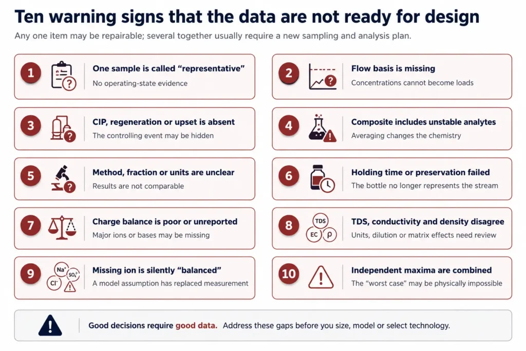
Data acceptance gateBefore the dataset enters technology screening or process modelling, confirm: the inference space is named; stable and event states are represented; sample type matches the decision; preservation and method requirements were met; flow and historian data are linked; blanks, spikes and replicates support the intended use; charge and physical cross-checks are coherent; missing ions remain explicit assumptions; and normal, design and worst-credible cases are physically possible.

7.12 Chapter conclusion

A single sample can describe one bottle under one operating condition. It cannot establish the distribution required to design a reliable MLD, ZLD or valorization system. The sampling programme must begin with the inference space and operating-state matrix, then select grabs, time composites, flow-proportional composites, event samples and continuous measurements according to the decision.

Preservation, holding time, sample fraction, method performance and quality-control samples determine whether the analytical result still represents the wastewater. Charge balance, conductivity, density, TDS, ion sums and process chemical ledgers provide independent diagnostics, but they do not authorize the silent reconstruction of missing chemistry.

The deliverable is a set of physically coherent normal, design, turndown and worst-credible compositions with uncertainty attached. Chapter 8 uses those cases to explain how concentration changes scaling, fouling, foaming and corrosion risk.

Chapter 7 in one sentence Design for distributions, not one sample: link every result to an operating state, a sampling basis, a quality-control record and a physically coherent decision case.