The correct economic metrics

Use the metric that answers the decision, with the denominator and time basis visible in every claim.

Controlled principle An economic metric is a compressed statement of a model, not the model itself. It is valid only when the numerator, denominator, system boundary, analysis period, price basis, discounting convention, availability and risk treatment are explicit. A favourable ratio cannot repair an incomplete business case.

Different decisions require different metrics

Chapter 28 handed forward a controlled option model: a counterfactual, a selected technical boundary, total project cost, life-cycle OPEX, avoided costs, qualified product value and downside cases. Chapter 29 does not add a single universal KPI. It selects a metric family according to the decision being made.

NIST life-cycle-cost guidance treats present-value life-cycle cost as the primary basis for comparing alternatives with different timing of initial and future costs, while supplementary measures such as net savings, return measures and payback answer narrower questions. HM Treasury’s 2026 Green Book likewise distinguishes present-value appraisal, cost-effectiveness measures and financial impacts rather than treating one ratio as sufficient.

Decision question	Primary use	Metric family	Main limitation
Operating control	What did the system cost and produce during the stated period?	Annual cost per actual feed, water recovered, residual eliminated or product.	Can hide future replacements and end-of-life cost.
Option comparison	Which alternative has the lowest complete cost for an equivalent service?	Present-value life-cycle cost or levelized unit cost.	Invalid if service, boundary or analysis period differs.
Investment decision	Does incremental value exceed incremental cost?	NPV / net present savings with downside cases.	Requires a defined counterfactual and cash-flow timing.
Return communication	How quickly and at what implied return is capital recovered?	IRR and simple/discounted payback as secondary indicators.	Can mis-rank alternatives or ignore later cash flows.
Environmental monetization	What monetary effect is assigned to GHG change?	Carbon cost or shadow carbon value on a stated emissions boundary.	Must not be confused with a market allowance price.

Table 29.1. Metric decision table: select the measure from the decision question, then expose its limits.

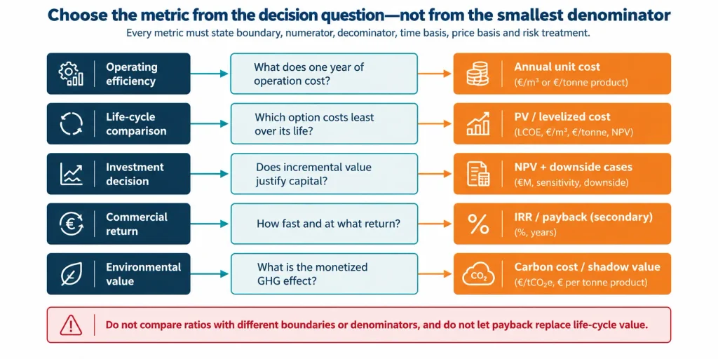
Figure 29.1. Metric decision map. A metric is chosen only after the decision question and accounting basis are defined.

Create a denominator register before calculating unit cost

The numerator can be identical while the reported result changes materially because the denominator changes. For this reason, each option should carry a denominator register that identifies the physical quantity, location, quality, time basis and exclusions. Nameplate capacity is not an acceptable substitute for actual annual throughput unless the metric is explicitly a capacity-normalized cost.

Denominator	Controlled definition	Required basis	Common error
Feed water / brine	Actual volume crossing the defined treatment boundary.	Average/design flow, density, operating hours, recycle treatment and downtime.	Using upstream plant capacity instead of actual brine feed.
Recovered water	Net water delivered to the named user after internal consumption and losses.	Quality specification, delivery point, availability and rejected/off-spec water.	Using gross distillate or membrane permeate.
Residual liquid eliminated	Baseline residual volume minus project residual liquid leaving the same boundary.	Baseline endpoint, project purge, cleaning waste, condensate reject and moisture carryover.	Calling concentration factor or water recovery ‘brine eliminated’.
Salt mass removed	Dissolved-solids mass removed from the stated liquid endpoint or immobilized in managed solids.	Ion/salt basis, density, reagents, precipitate water and closure error.	Using wet sludge or product mass as salt removed.
Qualified product	Saleable or internally accepted on-spec mass at the delivery point.	First-pass yield, rework, rejection, moisture, packaging loss and buyer acceptance.	Using contained inventory or gross crystals.
Service / production enabled	Incremental production or service protected by the project.	Causal link, capacity limit, contribution margin and downtime basis.	Crediting all site production to the water project.

Table 29.2. Denominator register for water, residual, salt, product and production metrics.

Use annual unit costs for operations—and levelized costs for life-cycle comparison

Annual unit cost is appropriate for a defined operating period when actual cost and actual output are known. It should separate fixed and variable cost, identify whether capital recovery is included, and use actual availability. It is not automatically comparable with a vendor’s design-year estimate or another project’s levelized cost.

Visible equations Annual unit cost = annual relevant cost ÷ annual actual quantity. Levelized unit cost = present value of relevant life-cycle cost (net of only the benefits assigned to that metric) ÷ present value of the corresponding physical output. Costs and output must use the same analysis period, timing convention and option boundary.

Metric	Numerator	Boundary control	Decision use
Gross treatment cost	CAPEX recovery + fixed OPEX + variable OPEX + replacement + residual management.	No avoided cost or product value deducted.	Shows the burden of operating the selected treatment boundary.
Net treatment cost	Gross treatment cost minus defensible avoided water, disposal, production and internal-substitution value.	Qualified product netback may be shown separately or deducted only with explicit convention.	Shows remaining owner burden after attributable value.
Levelized gross cost	PV of gross costs / PV of the selected quantity.	Discount rate, real/nominal basis and timing stated.	Compares alternatives with different cash-flow profiles.
Levelized net cost	PV of costs minus PV of attributable avoided costs and qualified value, divided by PV quantity.	No double counting; zero-revenue case retained.	Shows risk-adjusted unit burden, not a commodity production cost.
Marginal recovery cost	Incremental cost of the next recovery step / incremental output or residual reduction.	Compare adjacent technically feasible endpoints.	Reveals when the final recovery increment dominates economics.

Table 29.3. Gross, net, levelized and marginal costs answer different questions.

Keep price basis, discounting and escalation internally consistent

Present-value metrics require a dated price basis and a consistent relationship between inflation, escalation and discounting. The Green Book explains that real values should be discounted with a real discount rate and that inflation adjustment is distinct from discounting. NIST life-cycle-cost guidance similarly requires future costs, replacements, residual values and recurring expenses to be converted to a common present-value basis. [1,2,5]

Basis	Required treatment	Discounting rule	Control
Real analysis	Constant purchasing-power currency at a stated base date.	Real discount rate; only real relative-price changes modelled.	Best for comparing technical alternatives without general inflation noise.
Nominal analysis	Cash flows include general inflation and specific escalation.	Nominal discount rate consistent with the financing model.	Best for affordability, debt service and nominal budgets.
Mixed basis	Some cash flows nominal, others real, or discount rate inconsistent.	Not permitted without explicit conversion.	Creates false NPV and levelized cost.
Foreign currency	Exchange rate, date, hedging, import duties and local/foreign split stated.	Sensitivity or contractual basis required.	Avoids hiding currency exposure inside contingency.

Table 29.4. Price and discounting conventions must be consistent before cash flows are compared.

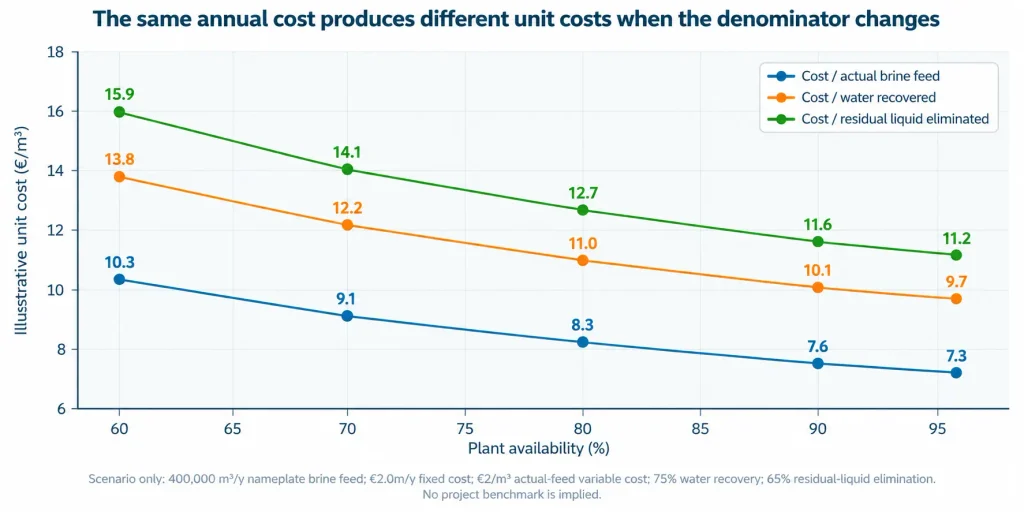
Figure 29.2. Scenario-only denominator and availability effect. The same cost model yields different unit costs because each denominator represents a different service.

Avoided cost is incremental value—not an accounting credit by default

Avoided cost is the expenditure or loss that the selected option prevents relative to the counterfactual. It is not the tariff, disposal fee or production value multiplied by theoretical output. The baseline contract, minimum charges, take-or-pay terms, fixed cost that remains, escalation and capacity constraints determine what is genuinely avoidable. EPA water-infrastructure guidance emphasizes life-cycle comparison of alternatives rather than isolated capital cost, and NIST guidance evaluates alternatives relative to a designated base case.

Avoided-cost route	Calculation basis	Required correction
Purchased water	Volume actually displaced × avoidable delivered cost.	Minimum purchase commitments, blending, backup supply and quality differences.
Residual disposal	Avoided tonnes/volume × avoidable transport and gate cost.	Fixed contract capacity, minimum haulage, classification and fallback storage.
Chemicals / utilities	Qualified internal product × substitution ratio × avoidable delivered purchase cost.	Purity adjustment, handling, losses, storage and supplier-contract minimums.
Production interruption	Expected reduction in lost contribution margin and restart cost.	Probability, duration, bottleneck, inventory buffering and double counting with reliability benefit.
Permit / liability exposure	Monetized only where a defensible expected-cost or provision basis exists.	Do not invent a probability or treat qualitative ESG benefit as cash.

Table 29.5. Avoided costs enter the model only to the extent they are incremental and avoidable.

Product value must remain qualification- and offtake-adjusted

Chapter 26 established that product value is reliable on-spec volume multiplied by delivered netback—not gross recovered mass multiplied by a headline price. Chapter 29 carries this into the economic model by separating physical yield, qualification probability, market placement, price basis and incremental product-train cost. A no-product-revenue case remains mandatory.

Risk-adjusted product value Expected product cash flow = reliable on-spec volume × placed fraction × delivered netback − incremental product finishing, QC, storage, logistics, off-spec and residual cost. Probability weighting may support decision analysis, but it does not convert an unsigned expression of interest into bankable revenue.

Status	Permitted economic treatment	Evidence boundary
Unqualified material	No revenue; residual or internal-development cost only.	Laboratory assay or theoretical yield.
Qualification in progress	Conditional scenario with explicit milestone and probability; base case may remain zero.	Buyer sample approval pending.
Qualified internal use	Avoided purchase value after substitution ratio and incremental handling.	Named user accepts delivered material.
Qualified external sale	Contracted/defensible delivered netback on accepted volume.	Specification, rejection, logistics and credit terms defined.
Hub / shared product	Value allocated after tolling, transfer price, losses and risk ownership.	Do not credit supplier and hub with the same margin.

Table 29.6. Revenue treatment follows qualification and contract evidence, not chemical recovery.

NPV is the primary investment metric; IRR and payback are supporting views

Net present value converts the project’s incremental cash-flow profile into one value at the selected discount rate. For mutually exclusive options, it preserves the scale and timing of cash flows and should remain the primary owner-financial decision metric. Public-sector or social appraisal may use different definitions, such as net present social value, and must not be mixed with the owner cash-flow NPV.

Metric	Definition	Use and warning
NPV / net present savings	Discounted incremental inflows minus outflows relative to the counterfactual.	Primary investment comparison when cash-flow boundary and discount rate are controlled.
IRR	Discount rate that sets NPV to zero.	Useful communication metric; can be ambiguous with non-conventional cash flows and can mis-rank mutually exclusive options.
Simple payback	Time until undiscounted cumulative net benefit recovers initial investment.	Liquidity screen only; ignores time value and later cash flows.
Discounted payback	Time until discounted cumulative net benefit recovers investment.	Improves timing treatment but still ignores post-payback value.
Benefit-cost / savings-investment ratio	PV benefits divided by PV costs under a defined convention.	Useful under capital constraints; can favour smaller projects and is sensitive to cost/benefit classification.

Table 29.7. NPV carries the complete cash-flow decision; return and payback metrics remain secondary.

NIST explicitly notes that payback measures ignore costs, savings and residual value after the payback date. A short payback can therefore coexist with a lower life-cycle value, while a longer-payback option can have the stronger NPV and operational resilience.

Treat availability and production interruption as economic variables

Availability affects both sides of the model: fixed cost is spread over less output, while water recovery, residual reduction and product placement decline. If the water or residual system constrains production, downtime may also create lost contribution margin, restart cost, emergency disposal or purchased-water cost. These effects must be linked to a causal event tree rather than added as a generic reliability premium.

Event	Economic basis	Control
Planned maintenance	Known frequency and duration; buffer/storage response.	Include planned lost output and maintenance cost once.
Unplanned outage	Probability × duration distribution × affected production/service.	Model emergency routes, restart and common-mode failures.
Feed-quality upset	Probability, treatment derating, off-spec product and disposal response.	Do not assume nameplate recovery under worst chemistry.
Buyer / disposal outage	Storage days, alternate route, curtailment threshold and cost.	Water plant must remain operable under zero-offtake case.
Production interruption	Affected line contribution margin, inventory protection, restart scrap and catch-up limits.	Use contribution margin, not gross sales, unless justified.

Table 29.8. Reliability value must be built from event probability, duration and consequence.

Carbon cost requires two separate steps: emissions accounting and valuation

First calculate the change in greenhouse-gas emissions against the counterfactual on a stated project boundary; then apply a selected market price, internal carbon price or shadow value. The GHG Protocol Project Accounting framework compares project emissions with a baseline, while current government conversion factors provide activity-to-emissions factors that must be dated and jurisdictionally appropriate. Carbon values used in appraisal are not the same as observed allowance prices.

Layer	Metric	Required distinction
Physical emissions	tCO2e by year from electricity, heat/fuel, chemicals, transport, construction, replacements and residuals as included.	Emission factors, geography, year and scope stated.
Market carbon cash cost	Allowances, taxes or contract charges actually paid.	Use applicable scheme and compliance boundary.
Internal carbon price	Company decision price applied consistently across options.	Corporate policy; not booked cash unless it creates expenditure.
Shadow carbon value	Monetary value used for economic appraisal of emissions impact.	Use the governing appraisal methodology and low/central/high cases.
Avoided emissions claim	Project minus credible baseline, including leakage and displaced activities.	Report separately from corporate inventory where required.

Table 29.9. Carbon accounting and carbon valuation are related but distinct economic layers.

ISO 14008 provides a transparency framework for monetary valuation of environmental impacts, and the World Bank’s 2024 guidance applies shadow carbon pricing in project economic analysis where GHG accounting is required. The correct value is therefore project- and institution-specific; this chapter introduces no universal €/tCO2e assumption.

Present a metric suite, not a single headline

Metric family	Minimum outputs	Control
Technical service	Actual feed; net recovered water; residual liquid eliminated; salt removed; on-spec product.	Annual and life-cycle quantities with availability.
Cost burden	Gross annual cost; gross levelized cost; marginal recovery cost.	No benefit deductions.
Owner value	Net treatment cost; NPV; cash requirement; debt-service/affordability view.	Incremental to counterfactual.
Return	IRR; simple and discounted payback; benefit-cost ratio where required.	Secondary to NPV and life-cycle cost.
Risk	P50/P90 or other stated cost range; downside NPV; switching values; break-even output/price.	Chapter 30 develops these.
Environmental monetization	Physical tCO2e plus market/internal/shadow carbon value.	Keep physical and monetary results side by side.

Table 29.10. Minimum metric suite for comparing MLD, ZLD and valorization options.

Economic-metric acceptance gate

A metric may enter decision material only when it can be reproduced from the controlled option model and compared on a common basis. Weighted scoring cannot compensate for a hidden denominator or inconsistent cash-flow boundary.

Gate field	Proceed	Conditional / recycle	Stop	Required record
Boundary	Source-to-endpoint scope and counterfactual are identical across options.	A minor interface allocation remains open.	Options omit different assets, residuals or benefits.	Boundary and option register.
Denominator	Physical quantity, quality, location, timing and availability are explicit.	Measurement plan is incomplete.	Nameplate or theoretical output is used without label.	Denominator register.
Cost basis	Gross/net convention, price date, currency and life-cycle items are explicit.	Some future cost timing requires refinement.	Equipment quote is treated as total or levelized cost.	Cost and cash-flow model.
Value basis	Avoided cost and product value are incremental, qualified and non-duplicative.	Conditional value is isolated from base case.	Headline price or non-avoidable tariff drives value.	Benefit ledger.
Investment metric	NPV and discount basis are stated; IRR/payback are secondary.	Financing structure is still provisional.	Payback alone selects the project.	Investment appraisal.
Reliability / carbon	Availability, interruption and GHG layers have explicit methods.	Scenario evidence remains limited.	Generic reliability premium or carbon price is inserted.	Risk and carbon registers.
Downside readiness	No-revenue, lower-availability and cost-escalation cases are calculable.	One downside needs more evidence.	Metric is valid only in optimistic case.	Chapter 30 handover.

Table 29.11. Economic metrics advance only when boundary, denominator, time and risk treatments are auditable.

Stop rule Stop or relabel any metric whose denominator, boundary, price basis or timing cannot be reconstructed. Do not compare €/m³ values that refer to different feeds, outputs, qualities, availability or life-cycle boundaries.

Handover to Chapter 30 — sensitivity and uncertainty

Chapter 30 tests which assumptions control the economic decision. It should receive the complete metric suite, not a single base-case result. Each metric must be linked to its input drivers, probability or scenario treatment, and decision threshold.

Handover field	Required basis for Chapter 30	Risk if missing
Selected decision metrics	Gross/net unit costs, levelized costs, NPV, IRR/payback and environmental monetization as applicable.	Sensitivity may optimize a secondary metric while the primary decision fails.
Denominator model	Flow, recovery, availability, residual reduction, salt/product yield and quality basis.	Output uncertainty is hidden inside the cost ratio.
Cost drivers	Energy, chemicals, replacement, labour, maintenance, transport, disposal and contingency timing.	Only CAPEX is varied.
Value drivers	Avoided water/disposal/production cost, product volume, netback, qualification and buyer placement.	Revenue downside is understated.
Financial basis	Analysis period, discount rate, inflation/escalation, tax, financing and currency.	Nominal and real cases are mixed.
Reliability / interruption	Event frequencies, durations, storage, emergency route and contribution margin.	Availability is a single unsupported percentage.
Carbon basis	Physical emissions by source and chosen market/internal/shadow value.	Carbon value changes without emissions sensitivity.
Thresholds	Switching values, covenant/affordability limits, maximum unit cost and minimum service requirements.	Sensitivity produces charts but no decision rule.

Table 29.12. Chapter 30 requires driver-linked metrics and explicit decision thresholds.

Chapter conclusion

Economic metrics are useful because they compress complex cash-flow and process models into decision signals. They are dangerous when the compression hides the physical service, time basis or risk boundary. Cost per cubic metre is meaningless until the reader knows which cubic metre; cost per tonne is meaningless until the material and moisture basis are defined; and payback is incomplete without the cash flows that occur after it.

The correct metric suite therefore combines physical service quantities, gross and net life-cycle cost, avoided cost, NPV, supporting return metrics, reliability exposure and transparent carbon valuation. Every result remains tied to the same counterfactual and source-to-endpoint boundary established in Chapter 28.

Chapter 30 now varies the drivers behind those metrics, tests mandatory downside cases and identifies the switching values that change the project decision.

Chapter 29 in one sentence The denominator, time basis and risk treatment must always be visible—because a favourable ratio is not evidence unless the underlying model is comparable and complete.