Sensitivity and uncertainty

A base case is a coordinate, not a forecast.

Controlled principle A base case is one internally consistent point, not a prediction. Sensitivity and uncertainty analysis are credible only when each range has evidence, linked variables change together where physics or contracts require it, and the results are tested against a stated decision threshold. Arbitrary symmetrical percentages and decorative tornado charts do not create risk-adjusted economics.

A base case is not the decision

Chapter 29 handed forward a controlled metric suite linked to the same counterfactual, physical denominators, cash-flow boundary and decision thresholds. Chapter 30 now asks which uncertain assumptions can reverse the preferred option, which combinations create an unmanageable downside, and which evidence or mitigation would change the answer. The objective is not to make uncertainty disappear. It is to show where it sits and whether the project remains defensible when reality differs from the central case.

HM Treasury’s 2026 Green Book requires sensitivity analysis and switching values for the preferred option and treats optimism bias, risk and uncertainty as explicit appraisal issues. GAO guidance similarly separates one-at-a-time sensitivity from combined risk and uncertainty analysis, and warns that unsupported plus-or-minus percentages are not a valid evidence base.

Term	Controlled meaning	Question answered	Common misuse
Base case	One internally consistent set of expected or central inputs.	What does the project look like under the selected central basis?	Treating it as the most probable or guaranteed outcome.
Sensitivity analysis	Recalculation after changing one driver at a time, while others remain fixed unless logically linked.	Which input has the greatest leverage on the decision metric?	Calling every high/low case a probability.
Scenario analysis	A coherent bundle of related assumptions describing a plausible operating, market or delivery state.	What happens when several linked conditions occur together?	Stacking unrelated worst values without a causal narrative.
Risk event analysis	Probability and consequence of a discrete event, with prevention and response.	What is the exposure to an identifiable event such as buyer loss or outage?	Hiding recurring variability inside a one-off risk event.
Probabilistic uncertainty analysis	Joint propagation of supported input distributions and dependencies through the model.	What range and confidence profile surround the output?	Using Monte Carlo to manufacture precision from weak inputs.
Optimism bias	Systematic tendency to understate cost/time and overstate benefits.	Is the central case biased before project-specific risks are added?	Applying a generic uplift and then double-counting the same quantified risks.

Table 30.1. Sensitivity, scenarios, risk and probabilistic uncertainty answer different questions.

Build a driver and dependency register before varying inputs

Sensitivity begins with a model map, not with the chart. Every decision metric should be traced to the physical, technical, commercial and financial inputs that create it. Each driver needs an owner, unit, base value, evidence source, date, range basis and dependency rule. The register should distinguish variables the project can control from external variables it can only monitor or contract around.

Driver family	Representative inputs	Required dependency	Primary decision effect	Owner / evidence
Hydraulic and production	Feed flow, campaigns, operating hours, expansion profile.	Flow must remain linked to actual production, storage and availability.	Plant sizing, annual output, fixed-cost dilution and residual load.	Owner production plan; reconciled water balance.
Feed chemistry	Major ions, scaling species, organics, temperature, density and variability.	Chemistry changes speciation, pretreatment, recovery limits, energy and solids together.	Train feasibility, reagent duty, cleaning, yield and downtime.	Sampling programme, laboratory QA and process model.
Process performance	Stage recovery, rejection, evaporation duty, crystallizer yield, product quality.	Water, salt, energy and residual balances must close after each change.	Unit cost, residual elimination, product volume and specification.	Vendor guarantee, pilot or calibrated model.
Asset life and reliability	Membrane/media life, cleaning frequency, maintenance, redundancy, ramp-up.	Replacement and downtime must affect both cash flow and denominator.	OPEX, availability, output and interruption exposure.	O&M basis, references, failure history.
Utilities and consumables	Electricity, steam/heat, chemicals, fuel, wash water.	Price and consumption are separate variables; load may change with chemistry and recovery.	Variable OPEX and carbon footprint.	Utility contracts, quotations and mass/energy balance.
Residuals and logistics	Disposal gate fee, transport, payload, storage, rejection and backup route.	Volume, classification, moisture and distance must change together.	Baseline avoided cost, fallback cost and operability.	Permits, carriers, disposal contracts and tests.
Product and offtake	Qualified yield, price/netback, placement fraction, buyer downtime, qualification delay.	Only qualified, deliverable volume earns value; unsold mass retains a cost.	Revenue, working capital, storage and downside viability.	Qualification record, contract and market analysis.
Capital and schedule	Total project cost, contingency, construction duration, commissioning and escalation.	Schedule changes timing, escalation, financing and benefit start.	NPV, affordability and contingency requirement.	WBS estimate, schedule and risk register.
Financing and macro	Discount rate, debt terms, currency, inflation/escalation and carbon value.	Real/nominal and currency bases remain internally consistent.	Present values, financing headroom and option ranking.	Finance basis and dated external assumptions.

Table 30.2. Driver register: sensitivity starts by mapping the model, dependencies and evidence owners.

Define ranges from evidence—not symmetrical percentages

A range should explain what could make the input low or high. GAO guidance states that sensitivity ranges should be traceable to data and assumptions rather than arbitrary percentage changes. UK infrastructure cost guidance uses reasonably optimistic, most-likely and reasonably pessimistic positions and expects the range to narrow as project maturity improves.

Ranges are often asymmetric. Energy price may have a contractual floor but an exposed upper tail; availability cannot exceed one hundred per cent but may fall sharply during ramp-up; feed chemistry may have distinct production modes rather than a continuous normal distribution; and product revenue can fall to zero even when price volatility appears modest. These shapes should remain visible instead of being forced into a symmetric low/base/high template.

Evidence state	Range basis	Permitted treatment	Do not do	Next evidence
Operating history	Observed distribution by stable mode, season, campaign and upset.	Use empirical percentiles or bounded mode-specific scenarios after data QA.	Pool incompatible production modes into one average distribution.	Extend monitoring where tails or correlations are poorly observed.
Comparable reference	Comparable chemistry, scale, duty, duration and maintenance basis.	Use transferred range with explicit adjustments and residual uncertainty.	Use a vendor headline from a different feed or system boundary.	Obtain reference data or independent review.
Pilot / demonstration	Representative feed, recycles, upsets, cleaning and output quality.	Use measured range within the demonstrated envelope; retain scale-up uncertainty.	Treat a short stable run as full availability or life evidence.	Longer integrated test and scale-up assessment.
Quotation / contract	Dated scope, exclusions, price basis, validity and indexation.	Use contractual bounds where enforceable; separate quantity from price uncertainty.	Treat a budget quote as fixed total project cost.	Firm bid, commercial terms and interface closure.
Engineering judgement	Structured expert basis with assumptions and comparable evidence.	Use a documented range and confidence label; test wide scenarios.	Insert an unexplained ±10% or ±20%.	Target the missing analysis, sample or quotation.
Unknown / emerging issue	No defensible distribution or bounded range yet.	Use explicit scenario branches, stop rules or [EVIDENCE REQUIRED].	Assign a precise probability to close the model.	Investigation, pilot, legal review or market qualification.

Table 30.3. Range construction must reveal the evidence state and the reason for asymmetry.

One-way sensitivity identifies leverage—not combined probability

One-way sensitivity changes one driver between supported low and high values and recalculates the selected metric while other independent inputs remain at base. The result identifies leverage: the variables whose uncertainty most changes NPV, life-cycle cost, unit cost, affordability or another selected decision threshold. It does not state the likelihood of the low or high result, and it does not represent several drivers moving together.

Step	Required action	Control question	Output
1. Select metric	Use the primary metric and threshold handed from Chapter 29.	Would a favourable secondary KPI hide failure of the primary decision?	Base metric and decision rule.
2. Select drivers	Prioritize material, uncertain inputs and explicit assumptions.	Does the driver affect the numerator, denominator or both?	Sensitivity test list.
3. Set evidence-based bounds	Record low/base/high or named discrete values and their source.	What physical, contractual or market condition creates each bound?	Auditable range register.
4. Preserve dependencies	Change directly linked quantities together; otherwise hold inputs fixed.	Does the change violate mass balance, process physics or contract logic?	Reconciled model run.
5. Recalculate	Run each driver independently and record the metric change.	Can the run be reproduced without manual formula edits?	Low/base/high outputs.
6. Rank and interpret	Order by decision impact and identify switching values.	Is the driver uncertain, controllable and decision-critical?	Tornado, mitigation priority and evidence plan.

Table 30.4. Credible one-way sensitivity keeps the model boundary and dependency logic intact.

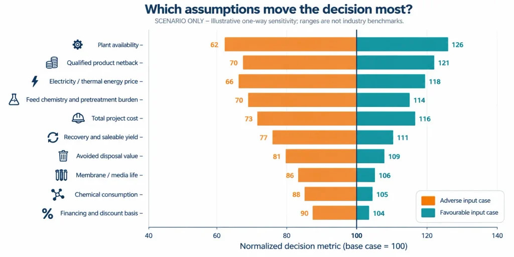
Figure 30.1. Scenario-only tornado chart. Bar length shows one-way leverage on a normalized decision metric; it does not show probability or a universal ranking.

Interpretation rule A long tornado bar is not automatically the highest risk. Decision priority depends on four things together: impact, uncertainty, controllability and time to act. A large but contractually fixed energy price may require monitoring rather than redesign; a moderately sensitive but poorly known feed impurity may justify immediate sampling or pilot work.

Technical sensitivity must preserve process physics and mass balance

MLD, ZLD and valorization inputs are coupled. A recovery change affects concentrate flow, ionic strength, scaling potential, energy, chemical consumption, solids production, product yield and availability. A poorer-feed case may lower membrane recovery, add pretreatment, shorten cleaning intervals and alter product qualification simultaneously. Sensitivity runs that change only the economic cell while leaving the process model untouched are not valid technical cases.

Technical driver	What must change with it	Required outputs	Failure signal
Feed flow / campaign	Hydraulic loading, operating hours, storage, turn-down, fixed-cost allocation.	Annual feed, product water, residual and availability by mode.	Nameplate flow rises but utilities, storage and downtime remain unchanged.
Feed chemistry	Speciation, saturation, pretreatment dose, solids, membrane/thermal duty and materials risk.	Revised water/salt/reagent balance and operating envelope.	TDS changes alone while ionic composition and fouling remain fixed.
Water recovery	Concentrate flow/composition, pressure or thermal duty, cleaning, purge and product-water quality.	Net water, residual eliminated, SEC and residual destinations.	Recovery increases without additional energy, scale or residual burden.
Membrane / media life	Replacement quantity, downtime, inventory, labour and disposal.	Life-cycle replacement cost and lost output.	Only replacement purchase cost changes; outage and denominator do not.
Chemical consumption	Reagent price and purity, by-product ions, sludge mass, handling and storage.	Dose, residual chemistry, solids and variable OPEX.	Dose changes without downstream ionic or sludge effects.
Availability	Planned and forced outage, ramp-up, start/stop losses, storage and backup route.	Annual service, fixed-cost dilution and interruption consequence.	Availability changes revenue but not water or residual service.
Product yield / quality	Recovery, washing loss, rework, off-spec fraction, qualification and disposal.	Qualified volume, residual mass and netback.	Chemical capture is varied as if every tonne remains saleable.

Table 30.5. Technical sensitivities must recalculate the process and residual system—not only the spreadsheet output.

Mandatory downside scenarios test whether the water project can continue

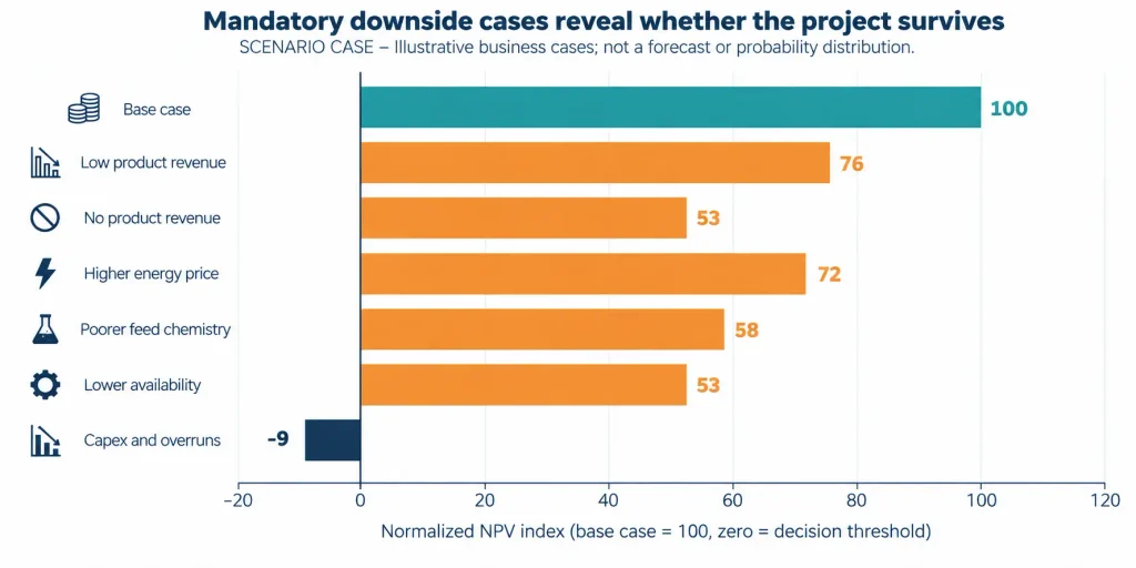
The master specification requires low-revenue, no-revenue, higher-energy, poorer-feed and lower-availability cases. These are not optional investor illustrations. They test whether the treatment and residual-management obligation remains operable when the optimistic commercial or operating assumptions fail. The no-product-revenue case must retain all costs and liabilities that remain when sales disappear, including product finishing that cannot be bypassed, storage, rejected material and the compliant fallback route.

Scenario	Minimum change from base	Must remain in the model	Decision question
Low product revenue	Lower placement fraction and/or delivered netback; qualification timing may slip.	Unsold output, storage, working capital, rework and fallback disposal.	Does limited commercial value still justify the product train?
No product revenue	External sales set to zero; internal value only if physically and operationally proven.	Residual handling, contractual obligations and any unavoidable finishing cost.	Can the core water/residual project operate lawfully and affordably?
Higher energy	Supported electricity and thermal price or consumption downside.	Linked carbon, capacity charges, demand peaks and process duty.	Does variable OPEX or utility capacity reverse the option?
Poorer feed	Adverse but credible chemistry, variability or contaminant event.	Pretreatment, recovery limits, cleaning, solids, quality and corrosion effects.	Is the design robust outside the average analysis?
Lower availability	Longer ramp-up, more cleaning, forced outage or reduced spares support.	Fixed cost, annual denominator, backup storage and production interruption.	Can the service objective be maintained with realistic uptime?
Cost and schedule escalation	Higher total project cost and later commissioning / benefit start.	Escalation, financing, contingency, temporary disposal and owner cost.	Does delay or capital growth destroy affordability or NPV?
Compound downside	A coherent bundle of the most credible interacting downsides.	Correlations, timing and mitigations; no double counting.	Where is the practical failure boundary of the preferred option?

Table 30.6. Mandatory downside cases protect the treatment obligation from optimistic operating and product assumptions.

Scenarios must be coherent bundles, not stacks of arbitrary lows

A scenario describes a plausible state of the project and its environment. Variables should move together only when a causal, physical or contractual relationship exists. For example, poorer feed may increase chemical use, reduce recovery, shorten membrane life and lower product quality; a buyer outage may reduce placement while increasing storage and disposal; a construction delay may increase escalation, temporary disposal and financing while postponing benefits. Conversely, unrelated pessimistic assumptions should not be combined simply to create an extreme result.

Scenario element	Consistency test	Valid linkage example	Invalid linkage example
Narrative	Can the bundle be described as a credible operating, market or delivery state?	Seasonal production campaign causes high flow and a known impurity peak.	All inputs are set to their lowest value with no common cause.
Timing	Do changes occur in the same period and for a credible duration?	Buyer outage coincides with storage accumulation and temporary disposal.	Lifetime product price is reduced because of a one-month outage.
Physical dependency	Does process physics require inputs to move together?	Higher sulfate lowers recovery and increases precipitation solids.	Electricity price changes membrane rejection.
Commercial dependency	Do contract terms link volume, price, quality or schedule?	Off-spec delivery triggers rejection, return freight and lower placement.	Global benchmark price changes internal avoided-water value.
Mitigation	Are prevention and response costs included and benefits adjusted?	Additional storage reduces shutdown probability but adds CAPEX and losses.	Risk probability falls without adding the mitigation asset or operating cost.
Comparison symmetry	Are all options exposed to the same external state?	Every option uses the same energy-price and production-demand scenario.	Only the preferred option receives the favourable market case.

Table 30.7. Scenario logic must be causal, timed and symmetrical across alternatives.

Use probabilistic analysis only when inputs and dependencies justify it

Probabilistic analysis combines several uncertain variables and recalculates the model repeatedly to create an output distribution. GAO and UK infrastructure guidance identify Monte Carlo simulation as a common technique for quantitative risk and uncertainty analysis, but both emphasize supported input ranges, appropriate distributions and dependencies. Correlation matters: treating energy consumption and availability, feed severity and chemical use, or construction duration and cost escalation as independent can materially understate or distort the tail.

A probabilistic model is not automatically superior to a scenario model. Where data are sparse, operating modes are discrete, legal outcomes are unresolved or the process is outside its demonstrated envelope, transparent scenarios and stop rules may be more honest than smooth probability distributions. The model should label epistemic uncertainty—what is not yet known—separately from operational variability that has been observed.

Input type	Possible representation	Minimum basis	Key caution
Observed continuous variability	Empirical or fitted bounded distribution.	Quality-controlled observations from relevant operating modes.	Do not extrapolate tails beyond the process envelope without justification.
Minimum / most likely / maximum	Triangular or another justified bounded form.	Expert-elicited points supported by evidence and definition.	Convenience does not make a triangular distribution true.
Bounded without central mode	Uniform only when values are genuinely equally plausible.	Defensible lower and upper bounds.	Uniform distributions often conceal ignorance.
Discrete operating mode	Weighted discrete branches or separate scenario model.	Mode frequency, duration and transition evidence.	Do not average incompatible chemistry or availability states.
Risk event	Occurrence model plus consequence distribution.	Probability, trigger, duration, response and residual impact.	Avoid double counting the event in both base range and risk register.
Contract / legal outcome	Discrete branches until terms or approval are resolved.	Defined alternatives and consequences.	Assigning a precise probability may create false confidence.
Correlated inputs	Joint sampling, conditional logic or common driver.	Causal evidence and direction/strength of dependency.	Ignoring correlation can narrow or shift the output distribution.

Table 30.8. Probability distributions are evidence statements, not formatting choices.

Output	Controlled interpretation	Useful decision	Do not claim
Probability distribution	Modelled range of outcomes under stated inputs, dependencies and iterations.	Compare alternatives and identify tail exposure.	A forecast outside the defined model and evidence boundary.
Percentiles / confidence points	Output value not exceeded—or exceeded—at the stated orientation and probability.	Set contingency, affordability or service confidence targets.	A universal P-value or one confidence level appropriate to every owner.
Expected value	Probability-weighted mean under the model.	Portfolio or repeated-decision view where appropriate.	A guaranteed or “most likely” outcome.
Median	Midpoint of the modelled output distribution.	Communicate a central probabilistic outcome.	Automatically the budget, contract price or target.
Tail / failure probability	Share of runs breaching a defined cost, NPV, capacity or service threshold.	Assess resilience and mitigation need.	A meaningful result without a pre-agreed threshold.
Correlation / contribution	Statistical relationship between sampled inputs and output.	Identify combined uncertainty drivers.	Causation without engineering interpretation.

Table 30.9. Probabilistic outputs require an orientation, threshold and decision use.

Switching values convert sensitivity into decision rules

A switching value is the input value at which the decision changes—for example, NPV reaches zero, the selected option becomes more expensive than the lower-complexity alternative, the unit cost exceeds an affordability limit, or residual service falls below the minimum requirement. HM Treasury requires switching values because they show how much an assumption must move before the apparent preference disappears. [1]

Switching-value test For each decision-critical driver, solve for the value at which the primary threshold is crossed. Then compare that value with the evidence-based range, contract position and monitoring trigger. A switching value that lies inside normal variability is a warning; one far outside a credible range is evidence of resilience, not proof that every other risk is controlled.

Decision threshold	Example switching question	Required comparison	Management response
NPV = 0	At what energy price, CAPEX or product netback does incremental NPV become zero?	Switching value versus contract range, forecast and downside scenario.	Hedge, redesign, secure price terms or stop.
Option ranking changes	At what availability or recovery does MLD become preferable to ZLD?	Switching value versus demonstrated operating envelope.	Select lower-complexity option or de-risk performance.
Affordability / funding cap	At what total project cost or schedule does funding headroom fail?	Switching value versus probabilistic cost and contingency.	Re-scope, stage, obtain funding or reject.
Maximum unit cost	At what annual output or downtime does €/m³ exceed the owner limit?	Switching output versus production and reliability cases.	Add redundancy/storage or revise service objective.
Minimum residual service	At what feed severity or outage does compliant residual capacity fail?	Switching point versus design/upset chemistry and storage duration.	Increase fallback capacity or stop the option.
Product-train justification	At what qualified yield or placement does incremental product NPV become negative?	Switching value versus qualification and offtake evidence.	Remove, modularize or defer product train.

Table 30.10. Switching values connect model sensitivity to monitorable design, contract and stop conditions.

Use sensitivity to choose mitigation and the next evidence

The analytical output should change project action. A sensitive and uncertain technical driver may justify sampling, modelling or pilot work. A sensitive market driver may justify an internal-use route, floor-price structure, take-or-pay commitment or modular product train. A sensitive reliability driver may justify redundancy, spares, emergency storage or a lower recovery target. Mitigation should be modelled with its cost, implementation time and residual risk; otherwise the project receives free risk reduction.

Evidence gathering should be proportional to decision leverage. The highest-value investigation is not necessarily the largest technical unknown. It is the unresolved input whose credible range crosses the decision threshold and whose uncertainty can be reduced before commitment. Where no practical evidence can close the uncertainty, the appropriate response may be optionality, staged investment, contractual transfer or rejection of the concept.

Driver condition	Preferred response	Cost / burden to include	Closure evidence
High impact, high uncertainty, reducible	Targeted sampling, pilot, reference check, quotation or legal/commercial diligence.	Test programme, schedule and owner effort.	Narrowed range and updated switching comparison.
High impact, contractible	Fixed/indexed utility terms, performance guarantee, price floor, take-or-pay or capacity reservation.	Premium, security, exclusions, credit and counterparty risk.	Executed term and residual exposure.
High impact, design-controllable	Redundancy, storage, bypass, modularity, lower recovery or alternate residual route.	CAPEX, OPEX, footprint, complexity and new failure modes.	Revised design and demonstrated operability.
High impact, not controllable	Stage investment, preserve optionality, set monitoring trigger or stop.	Delay, option premium and interim residual cost.	Decision gate and trigger owner.
Low impact, high uncertainty	Monitor; avoid expensive investigation unless dependency changes.	Monitoring and model maintenance.	Periodic review.
Mitigation exceeds avoided exposure	Accept within risk appetite or reject the option.	Residual risk and contingency.	Owner approval and risk allocation.

Table 30.11. Sensitivity becomes valuable only when it directs evidence, mitigation, optionality or a stop decision.

Govern the model as a living decision record

Sensitivity and uncertainty results expire when the feed, design, quotations, contracts, schedule or market basis changes. The model should therefore be version-controlled and reconciled to the current mass balance, estimate and risk register. Every input needs a source date and owner; every scenario needs a definition; every correlation or conditional rule needs a rationale; and every output needs its threshold and orientation. The Orange Book and ISO 31000 both frame risk management as an integrated, continually improved part of decision-making rather than a one-time appendix.

Control	Minimum record	Review trigger	Failure prevented
Input register	Value, unit, source, date, range, evidence state and owner.	New data, design change, quotation expiry or contract revision.	Orphan assumptions and silent overwrites.
Dependency register	Formula links, correlations, conditional logic and physical rationale.	Process redesign, new operating mode or risk event.	Impossible combinations and understated tails.
Scenario register	Narrative, changed inputs, timing, duration, mitigation and comparison symmetry.	New credible downside or owner decision.	Unreproducible “best/worst case” bundles.
Model assurance	Units, formulas, mass/cost reconciliation, duplicate benefits and error checks.	Every material revision and stage gate.	Charts generated from a broken or inconsistent model.
Decision thresholds	NPV, affordability, service, permit, capacity and risk appetite limits.	Governance or financing change.	Analysis without a decision rule.
Actual-versus-model update	Operating, cost, schedule, quality, reliability and market outturn.	Pilot, commissioning and routine operations.	Repeated optimism and stale uncertainty ranges.

Table 30.12. The uncertainty model must remain traceable, reviewable and updateable through project development.

Sensitivity and uncertainty acceptance gate

The project may advance only when the critical drivers, downside cases and switching thresholds are visible enough to support a decision. A sophisticated simulation cannot compensate for an unqualified product, an absent residual route, a broken mass balance or an undefined counterfactual.

Gate field	Proceed	Conditional / recycle	Stop	Required record
Model and metrics	Controlled model reproduces Chapter 29 metrics on a common boundary.	Minor reconciliation or audit issue remains.	Sensitivity is performed on disconnected or inconsistent calculations.	Model-assurance record.
Ranges	Material ranges are evidence-based, asymmetric where needed and owned.	Some secondary ranges rely on documented judgement.	Critical ranges are arbitrary or unsupported.	Driver and range register.
Dependencies	Physical, schedule, commercial and financial links are modelled.	One dependency awaits evidence and is bounded by scenarios.	Mass balance, correlations or conditional effects are ignored.	Dependency map.
Mandatory downsides	Low/no revenue, higher energy, poorer feed and lower availability are operable cases.	One case requires further design or contract evidence.	Water/residual service fails without optimistic revenue or uptime.	Downside scenario pack.
Probabilistic analysis	Method is proportionate; distributions and correlations are supported.	Scenario analysis used transparently because data are limited.	Precise probabilities are invented to force a confidence result.	Uncertainty-method statement.
Switching values	Decision-critical thresholds are calculated and compared with credible ranges.	One switching value depends on unresolved commercial/legal evidence.	Charts show movement but no condition that changes the decision.	Switching-value register.
Mitigation and ownership	Actions, costs, residual risk, triggers and owners are defined.	Further evidence has a dated owner and gate.	Risk reduction is assumed without cost or responsibility.	Risk treatment and evidence plan.

Table 30.13. Sensitivity and uncertainty analysis advances only when it can change or defend the project decision.

Stop rule Stop, simplify or re-stage the project when the preferred case fails under a credible mandatory downside, when a switching value lies inside normal variability without a mitigation, or when the water and residual obligation depends on uninterrupted product sales. Do not use a Monte Carlo confidence percentile to hide an unresolved fatal assumption.

Handover to Chapter 31 — environmental assessment

Chapter 31 compares physical environmental burdens rather than assuming that higher recovery is automatically better. It should receive the base, mandatory downside and selected probabilistic or scenario outputs for water, electrical and thermal energy, chemicals, solids, residual classifications, transport and greenhouse-gas emissions. Environmental comparison must use the same feed, operating hours, availability, product qualification and residual endpoints as the economic cases.

The handover should expose which environmental results are sensitive to feed severity, recovery, energy source, chemical dose, solids moisture, product rejection, transport and disposal fallback. Monetary carbon values may accompany the physical inventory, but Chapter 31 must retain physical units and cross-media impacts even when they are not monetized.

Handover field	Required basis for Chapter 31	Environmental risk if missing
Scenario set	Base, higher-energy, poorer-feed, lower-availability, no-product and compound cases.	Environmental comparison reflects only the optimistic operating state.
Water balance	Feed, net recovered water, internal consumption, residual liquid, evaporation and losses.	Recovery claims use inconsistent denominators.
Energy inventory	Electrical and thermal energy by block, source, quality and operating case.	Carbon and cross-media burdens are hidden or double counted.
Chemical and consumable inventory	Reagent type, purity, dose, upstream burden where available, membranes/media and cleaning.	Chemical substitution and secondary salt loads are omitted.
Solids and residuals	Dry/wet mass, moisture, composition, classification, leachability need and destinations.	Liquid reduction is credited while solid burden disappears.
Products and rejected output	Qualified volume, internal substitution, off-spec, unsold mass and fallback.	Avoided impacts are credited to production that is not used or sold.
Transport and infrastructure	Payload, distance, mode, storage, return trips, shared assets and lifetime.	Hub or product logistics are outside the environmental boundary.
GHG and valuation	Physical tCO2e by source plus separately stated market/internal/shadow value.	A monetary carbon value replaces the emissions inventory.
Environmental thresholds	Permit, water-risk, hazard, land, air and owner sustainability constraints.	A lower cost option advances despite an unacceptable environmental condition.

Table 30.14. Chapter 31 requires scenario-linked physical inventories, not a single base-case recovery number.

Chapter conclusion

Sensitivity analysis identifies leverage by changing one supported input at a time. Scenario analysis tests coherent combinations such as poorer feed, higher energy, lower availability and buyer loss. Probabilistic analysis can then quantify combined uncertainty where distributions and dependencies are defensible. Each method has a different purpose and none replaces the need for a controlled physical and economic model.

The mandatory commercial test is the no-product-revenue case. The mandatory technical tests include poorer feed and lower availability. The decisive output is not the chart itself but the switching value, failure threshold, mitigation and owner. A project is resilient when the critical thresholds remain outside credible ranges or when practical, costed actions keep the treatment and residual obligation operable.

Chapter 31 now tests whether the economically resilient options also minimize total environmental burden without shifting impacts from liquid discharge into energy, chemicals, solids, transport or hazardous residuals.

Chapter 30 in one sentence A project is decision-ready only when its critical assumptions, coherent downside cases, switching values and mitigation actions are explicit—and the water and residual system survives without product revenue.